

You may be familiar with Microsoft Excel. This application made by Microsoft Corporation is the application with the most users in the world in 140+ countries. This application has a myriad of Excel formulas that can accurately present numbers and data.
The primary function of Microsoft Excel is calculation, which is why it has been used by many users, both students and office workers. Despite other spreadsheet programs (competitors), Excel maintained its dominance and even became an industry standard.
Apparently, Excel seems too good to be true. All you have to do is enter an Excel formula, and almost everything you need to do manually can be done automatically. Use the best accounting software to do the cash flow forecast appropriately and analyze financial statements more optimally.
If you need to combine two sheets with the same data, Excel can do this. Do you need help with mathematics? Excel can do this. Are you using data from multiple cells? Excel can do this too.
In this article, you will understand the function of Excel in different professional fields. Then you’ll understand what formulas you need to know. Later, you will be able to apply automatic calculations to be used according to your needs.

The Uses of Excel in Professional Fields
Many job openings require candidates to master Excel. Not surprisingly, excel is needed by a wide variety of fields of work that require data collection.
To that end, we will present the following professions, which can benefit from the use of Excel, among others:
Accountancy
It is widespread for accountants to be able to use Excel. The field of accounting benefits from using Microsoft Excel in several ways, including making it easier to calculate corporate profit and loss, identify large profits over a period, calculate employee salaries, and more.
An accountant can facilitate his work by using the accounting system as a tool he worked. The system can provide convenience in managing the company’s financial circulation and calculating it optimally and accurately.
Also Read: Salary Slip: Understanding, Benefits, Format, Example
Mathematical calculations
The next advantage of using Microsoft Excel is mathematical calculations. Use calculations to find data from numbers, subtractions, multiplications, and divisions, as well as various other variations such as calculating the slope.
Data processing
In data management, there are helpful excel formulas, including managing statistical databases, calculating data, searching for median values, and averages, and searching for the maximum and minimum values of data sets.
Graphic creation
Excel allows you to create graphics. Such as graphing population development data for one year, the graph of student library visits for one year, the student graduation graph for six years, the graph of student number development for three years, and others.
Table operations
The last application is to be able to operate the table. With a total of 1,084,576 rows and 16,384 columns in Microsoft Excel, it will make it easier for you to enter data that requires a large number of columns and rows.
Complete Excel Formulas with Their Functions
In addition to the functionality and use of Microsoft Excel mentioned earlier, operating this Excel program requires Excel formulas. Each formula has a different function that you can use for a specific need.
Here are the Excel formulas you need to know, among others:
| Formulas | Functional Description |
| SUM | Summing |
| AVERAGE | Looking for Average Values |
| AND | Finding Value by comparison and |
| NOT | Finding Value with Exceptions |
| OR | Finding Value by Comparison or |
| SINGLE IF | Looking for Values If Conditions ARE RIGHT/WRONG |
| MULTI IF | Finding Values If Conditions ARE RIGHT/WRONG With Many Comparisons |
| AREAS | View The Number of Areas (Range or Cells) |
| CHOOSE | View Selection Results Based on Index Numbers |
| HLOOKUP | Search for Data from a table organized in a horizontal format |
| VLOOKUP | Search for Data from a table arranged in an upright format |
| MATCH | Displays the position of a specific cell address |
| COUNTIF | Counting the Number of Cells in a Range with specific criteria |
| COUNTA | Counting the Number of Filled Cells |
| CEILING | Round the number up |
| FLOOR | Rounds numbers down |
| DAY | Looking for The Value of the Day |
| MONTH | Searching for the Value of the Moon |
| YEAR | Looking for Year Value |
| DATE | Get a Date Value |
| LOWER | Change text letters to lowercase |
| UPPER | Change Text Letters to UpperCase |
| PROPER | Change the Initial Character of the Text To UpperCase |
For more information about how to use the excel function formulas mentioned above, here is a detailed description, along with examples:
SUM
This Excel summation formula has the primary function of summing numbers in specific cells. However, it is also often used to complete a job or task quickly.
To use SUM, first create a summation table and enter the summation formula below. For example, =SUM(G8:H8), or as shown in the image below:

Then, if the SUM formula has been entered, press enters to specify the amount. As shown in the picture below:

AVERAGE
The primary function of the AVERAGE formula or the average formula in Excel is to find the average value of a variable. The trick is to create a table for grades and then enter the AVERAGE formula to determine the student’s grade point average. For example, =AVERAGE(D2:F2), as in the following image:

If you enter the AVERAGE formula, press enters to see the result, shown in the image below.

AND
The AND formula function generates a TRUE value if all previously tested arguments are correct or can return a FALSE value if all arguments or answers are incorrect.
To determine TRUE or FALSE, you must create a table and enter THE FORMULA AND. For example, =AND(G7>I7).
This technique is usually used to help fill out questionnaires or answer question columns to speed up the value-setting process.
NOT
The NOT formula has the opposite function of the AND formula because it produces TRUE if the condition tested is FALSE and FALSE if the condition tested is TRUE.
The first step is to create a table and enter the FORMULA NOT to find out the results. For example, as shown in the diagram below, =NOT(G7>J7).
OR
The OR is the following excel formula that will produce TRUE data if some given argument is correct. If all of the arguments presented are incorrect, the answer is FALSE.
A student’s average test score result is an example of how OR can use it in Excel. If it is less than 70, he must repeat the course; if it is greater than 70, the student graduates.
SINGLE IF
The IF function is to return a value that, when examined, is TRUE and another value that is visible as FALSE.
Not much different from the technique of using formulas in OR. It just seems more straightforward.
For example, when a student’s average grade is less than 75, that student does not graduate, and vice versa. How to create an IF formula is =IF(J8<75;” NOT GRADUATING”;” PASS”). To be clear, take a look at the following image:

After entering the formula, press enters, and the result will match what you ordered.

MULTI IF
This formula is a further lesson from SINGLE IF, but if SINGLE IF only uses only one condition with two options, The MULTI IF uses two terms and three options.
A Double/Multi FORMULA is a type of logic-IF formula consisting of 2 or more IF in formula writing. If a single IF only needs 1 IF, for example, =IF(B2=>=70;” Graduated”;” Failed”) then Double IF requires more than 1 IF, for example, =IF(B2>=70;” Good”;IF(B2>=50;” Enough”;” Less”)).
So that the full Excel formula will provide Syntax on Double / Multi IF, among others:
=IF(Logical_Test; Value_If_True;IF(Logical_Test; Value_If_True; Value_If_False))
AREAS
You can use the usability of AREAS if you want to calculate the number of areas you want to select. The AREAS formula can use the formula =AREAS(G6:K8).

The result is one area. The results are based on the example in the image of selecting only one range of cells.
CHOOSE
The primary function of a CHOOSE formula is to display selection results based on index numbers or sequences in reference (VALUE) that contain text, numeric, formula, or range names. The image below shows an example of how to write the CHOOSE formula.

Meanwhile, the results of the CHOOSE formula are shown in the image below.

HLOOKUP
The HLOOKUP function displays data from tables arranged horizontally. However, The arrangement of tables or data in the first row should be based on small to large sequences or raising them.
For example, the number 1,2,3,4… Or the letter A-Z. Sort by ascending the menu if you previously typed randomly. Cases like the ones listed below are examples.

=HLOOKUP(Cells that contain packet types; Range cell table details costs; The location of the data column you want to retrieve;0).
VLOOKUP
The primary function of the VLOOKUP formula is almost identical to the HLOOKUP formula; The difference is that the VLOOKUP formula displays data from tables arranged in an upright or vertical format. The requirement is that the first row of the data table is prepared in small to large order or up.
For example 1,2,3,4… Or the letter A-Z. For example 1,2,3,4… Or the letter A-Z. Sort through the Ascending menu if you previously typed randomly.
MATCH
The MATCH function is one of the components of an Excel formula that you can use to perform lookups or reference data searches.
The MATCH function works by finding the relative position of a value in a range or array and generating a number that is the index of the cell’s relative position that contains the value it is looking for.
The use of the Excel MATCH function must follow the syntax rules, namely MATCH(lookup_value, lookup_array, [match_type])
To better understand, understand the image below:

COUNTIF
COUNTIF is a helpful formula for counting the number of cells that have the same criteria. As a result, you no longer have to struggle with data sorting.
Assume you’re doing a survey. You want to know how many civil servants there are out of 20 respondents. As a result, you can use the following formulas:
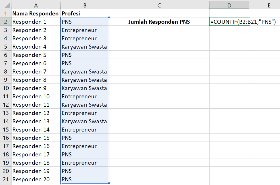
To get started, all you need to do is enter the range of cells you want to identify into the COUNTIF formula (B2:B21)
Then, enter the cell calculation criteria, namely “PNS” (must be in quotation marks).
This formula produces a result of 7. So, out of 20 respondents, seven were civil servants.
COUNTA
COUNTA has the function of counting the number of cells that contain numbers and the number of cells that contain anything. As a result, you can determine the number of cells that are not empty.
Assume that cells A1 through D1 are words and cells G1 through I1 number. Therefore the use of the formula is =COUNTA(A1:I1)

That results in 7 because the empty cells are only E1 and F1.
CEILING
The CEILING formula can round the number UP at the multiple values of a specific number. The formula is CEILING (CELLS number; Multiples).
Misalnya, CEILING(G9;100). Then the number on Cells G9 will be rounded up with a multiple of 100.
FLOOR
If the previous use of the formula is to round to the nearest integer and above, the FLOOR formula is used to round to the nearest integer. The formula is almost identical to the one for CEILING, but with the addition of FLOOR.
The FLOOR formula is FLOOR (Number cell; Multiples).


DAY
The DAY formula is used to find the date type data’s day (in the numbers 1-31). Consider the DAY function (column B). The date data in column A will be extracted and converted into numbers 1-31, following the explanation through the image:

After entering the formula =DAY(NUMBER), press enters and see the results below:

MONTH
Almost similar to the DAY formula, the use of the MONTH formula to search for months (in numbers 1-12) from date type data. For example, the use of the MONTH function (column K) of a column I date data, after extracting it, produces the numbers 1-12 as in the figure below:

YEAR
Meanwhile, there is a YEAR formula. The way you use this formula is similar to the way the previous two formulas were. The use of the YEAR formula takes years (in the range of 1900-9999) from date-type data.
DATE
The DATE formula has a function that allows you to get date data types by entering years, months, and days. The DATE function is the opposite of the DAY, MONTH, and YEAR functions, which describe month and year-type data from their respective dates.
Year, month, and day data in the form of numbers combined with the DATE function generate data with data types, as shown in the figure below. Date formula writing image, namely:

LOWER
The lower formula function converts all uppercase letters in the text to lowercase. To use the formula, type the LOWER command, and texts will convert the desired writing to lowercase.
For example, when implementing the LOWER formula with the formula =LOWER (Don’t Forget to Use HashMicro Software), the result is “don’t forget to use has micro software.”
UPPER
In addition to lower formulas, Microsoft Excel includes upper formulas. The use of UPPER is to convert all text containing lowercase letters into uppercase, the opposite of the LOWER function.
For example, if you type UPPER (hashmicro), your writing will be entirely in capital letters.
PROPER
Sometimes you forget to write sentences in all lowercase letters and no capital letters. So with the PROPER formula, you can capitalize on the first character in each word while keeping the rest. The formula is APPROPRIATE (text).
Conclusion
Although understanding Excel entirely takes time, you will be familiar with all the correct formulas and applications.
In a company, the use of Excel is overwhelming, especially in presenting data, statistics, and company finances such as salaries. The digital world is bringing corporate transformation to provide information and payroll more easily with automated systems. You can use HashMicro accounting software as a tool to calculate financial circulation optimally and accurately.
Moreover, HashMicro has a system that helps with all your human resource and employee administration tasks. With HashMicro’s HRM Software, calculates salaries, and manages leave and attendance lists, reimbursement processes, timesheets, and other operational activities in just seconds.
Produce reports accurately and comprehensively like thousands of large companies that have joined HashMicro. To check out more, click here.